Natural Distribution Function

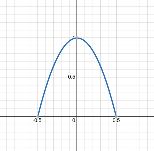
The Natural Distribution Function is a correction of the Normal Distribution Function.

The shape of the originally accepted curve assumes an infinite axial base, rather than a finite axial breadth. That breadth is related to one sample magnitude. Nature’s forces and related fields all evolve to displace matter according to square functions or simply parabolically distributed dimensions.

It is the assumption of an infinite horizontal axis which leads to the distorted (stretched) parabola of the classical, normal curve. The curve is a probability density curve where 1 is the greatest function value. Multiply it by a population or sample group to practically apply it.

f (x) = 1 - ( 2 * x ) ^ 2

Deviations From The Median Or From The Origin

Median: x = 6/6 --->

f (a) = 1.0000

1st deviation: x = 1/6 --->

f (a) = 0.8889

2nd deviation: x = 2/6 --->

f (a) = 0.5556

3rd deviation: x = 3/6 —->

f (a) = 0.0000

The area under the curve is

f (a) = 1 - ( 2 * ( 6/6 ) ) ^ 2 ,

-        3 ( the curve is negative )

For results which best obey BEDMAS, plot in Desmos.com or Geogebra.com  ( See the post about static BODMAS to BEDMAS™ Sequencing Law. )

See the post, The Photon/Particle Wave Function, for the equation’s place in the humble photon.

© Sydney Matinga 2026